PTT 與 Dcard 語料斷詞問題探討

這學期修了老闆的課──語料處理方法，認識了一個強大的 R 套件 zipfR (Evert and Baroni 2007) 以及 LNRE model (Baayen 2002)。這篇文章將參考老師的研究 (Hsieh 2014)，並依據 The zipfR package for lexical statistics: A tutorial introduction (Baroni and Evert 2014) 所提供的方法，以 PTT 與 Dcard 的語料進行中文斷詞問題的分析。

Introduction

在使用 zipfR 之前，要先認識 Zipf’s law (Zipf 1949)。簡單說明，即是在自然語言的語料庫中，一個單詞出現的頻率越高，在頻率表裡的排名越前面。且第一名的單詞出現的頻率大約是第二名單詞的兩倍、第三名單詞的三倍，以此類推。

接下來要了解 token 和 type 的意義。這裡有一個範例詞表：

蘋果, 橘子, 香蕉, 香蕉, 葡萄, 蘋果, 香蕉, 蘋果, 葡萄, 蘋果, 葡萄, 蘋果

這個詞表總共有 12 個 token (sample size = 12)，以及 4 個 type (vocabulary size = 4)。在這裡我們把它表示成

N = 12

V = 4

根據範例詞表，我們可以得到一個 type-frequency list：

接著，我們又可以得到一個 Zipf Ranking，這裡的 r 將頻率由大到小排序，fr 則是指頻率：

透過 type-frequency list，我們可以得到一個計算上非常重要的資料：frequency spectrum，其中 m 代表出現次數，Vm 代表出現該次數的單詞共有幾個：

在範例中，出現一次的單詞有一個 (橘子)，出現三次的單詞有兩個 (香蕉、葡萄)，出現五次的單詞有一個 (蘋果)。只出現過一次的單詞，我們稱之為 hapax legomena。

2. Lexical Richness

1
2
3
# 載入套件
library(readr)
library(zipfR)

首先，將平衡語料庫 (ASBC)、PTT 和 Dcard 語料匯入並整理。PTT 語料來自 2005、2010、2015，以及 2020 共四個年度的八卦板與女板，且對其進行抽樣。

 1
 2
 3
 4
 5
 6
 7
 8
 9
10
11
12
13
14
15
16
17
18
19
20
21
22
23
24
25
26
27
28
29
30
31
#asbc
asbc_corpus <- paste0(readLines("data\\asbc.txt", n=10000, encoding = 'UTF-8'),collapse=" ")
asbc_corpus <- unlist(strsplit(asbc_corpus, "\\s"))

# PTT Gossiping board (sampled)
g05 <- sample(readLines("data\\Gossiping_2005_seg.txt", encoding="UTF-8"), 1250)
g10 <- sample(readLines("data\\Gossiping_2010_seg.txt", encoding="UTF-8"), 1250)
g15 <- sample(readLines("data\\Gossiping_2015_seg.txt", encoding="UTF-8"), 1250)
g20 <- sample(readLines("data\\Gossiping_2020_seg.txt", encoding="UTF-8"), 1250)

g05 <- unlist(strsplit(g05, "\\s"))
g10 <- unlist(strsplit(g10, "\\s"))
g15 <- unlist(strsplit(g15, "\\s"))
g20 <- unlist(strsplit(g20, "\\s"))

# PTT WomenTalk board (sampled)
w05 <- sample(readLines("data\\WomenTalk_2005_seg.txt", encoding="UTF-8"), 1250)
w10 <- sample(readLines("data\\WomenTalk_2010_seg.txt", encoding="UTF-8"), 1250)
w15 <- sample(readLines("data\\WomenTalk_2015_seg.txt", encoding="UTF-8"), 1250)
w20 <- sample(readLines("data\\WomenTalk_2020_seg.txt", encoding="UTF-8"), 1250)

w05 <- unlist(strsplit(w05, "\\s"))
w10 <- unlist(strsplit(w10, "\\s"))
w15 <- unlist(strsplit(w15, "\\s"))
w20 <- unlist(strsplit(w20, "\\s"))

# PTT
ptt_corpus <- c(g05, g10, g15, g20, w05, w10, w15, w20)

# dcard
dcard_corpus <- readLines("data\\dcard_corpus.txt", encoding="UTF-8")

Type-frequency List

使用 zipfR 套件，可以簡單地得到 type-frequency list 和它的 Zipf ranking。為了進行接下來的比較，在這裡將套件內建的 Brown.tfl 一併匯入。

1
2
3
4
asbc.tfl <- vec2tfl(asbc_corpus)
data("Brown.tfl")
ptt.tfl <- vec2tfl(ptt_corpus)
dcard.tfl <- vec2tfl(dcard_corpus)

看一下資料的樣子。其中 k 代表 Zipf’s ranking，f 代表頻率，N 是 sample size，V 是 type count：

 1
 2
 3
 4
 5
 6
 7
 8
 9
10
11
12
head(ptt.tfl)

##    k    f type
## 的 1 3039   的
## 是 2 1578   是
## 我 3 1506   我
## 不 4 1123   不
## 了 5 1070   了
## 有 6  846   有
## 
##      N     V
##  77826 12837

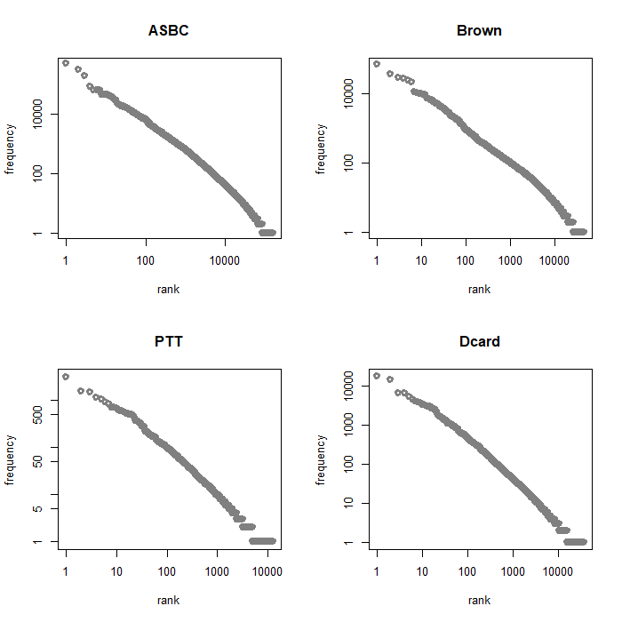
zipfR 也可以讓我們輕鬆將資料視覺化：

1
2
3
4
5
6
7
8
9
par(mfrow=c(2,2)) # 2*2 plot area
plot(asbc.tfl, main="ASBC", log="xy", # logarithmic scale
        xlab="rank", ylab="frequency")
plot(Brown.tfl, main="Brown", log="xy", 
        xlab="rank", ylab="frequency")
plot(ptt.tfl, main="PTT", log="xy", 
        xlab="rank", ylab="frequency")
plot(dcard.tfl, main="Dcard", log="xy",
        xlab="rank", ylab="frequency")

Frequency Spectrum

透過剛剛的 type-frequency list，我們可以得到 frequency spectrum。Brown corpus 的 frequency spectrum 可直接從套件中匯入：

1
2
3
4
asbc.spc <- tfl2spc(asbc.tfl)
data("Brown.spc")
ptt.spc <- tfl2spc(ptt.tfl)
dcard.spc <- tfl2spc(dcard.tfl)

看一下資料的樣子。此處的 m 是指出現次數，Vm 代表出現該次數的 type 共有幾個：

 1
 2
 3
 4
 5
 6
 7
 8
 9
10
11
12
head(ptt.spc)

##   m   Vm
## 1 1 7784
## 2 2 1850
## 3 3  777
## 4 4  481
## 5 5  267
## 6 6  209
## 
##      N     V
##  77826 12837

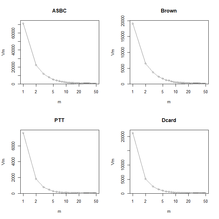
取 log 值後，下圖提供前五十筆 spectrum element 的資料：

1
2
3
4
5
6
7
8
9
par(mfrow=c(2,2))
plot(asbc.spc, log="x", main="ASBC",
        xlab="m", ylab="Vm")
plot(Brown.spc, log="x", main="Brown",
        xlab="m", ylab="Vm")
plot(ptt.spc, log="x", main="PTT",
        xlab="m", ylab="Vm")
plot(dcard.spc, log="x", main="Dcard",
        xlab="m", ylab="Vm")

從上圖可以得知，hapax legomena (只出現過一次的單詞) 占所有語料庫的比例都相當的高。接下來，我們可以透過 Vocabulary growth curves (VGC) 來觀察新詞增加的情況。

Vocabulary Growth Curves (VGC)

同樣地，透過 zipfR，我們可以將語料轉成 vgc object。Brown corpus 的資料一樣可以直接匯入：

1
2
3
4
asbc.vgc <- vec2vgc(asbc_corpus, m.max=2)
data("Brown.emp.vgc")
ptt.vgc <- vec2vgc(ptt_corpus, m.max=2)
dcard.vgc <- vec2vgc(dcard_corpus, m.max=2)

來看一下 ptt.vgc 裡面是什麼 :

1
2
3
4
5
6
7
8
9
head(ptt.vgc)

##      N    V  V1  V2
## 1    1    1   1   0
## 2  392  272 221  30
## 3  783  505 412  49
## 4 1174  711 566  73
## 5 1565  906 723  87
## 6 1956 1080 849 113

以 row 2 為例，表示在前 392 個 token 中，共有 272 個 type，而在其中有 221 個單詞只出現過一次。

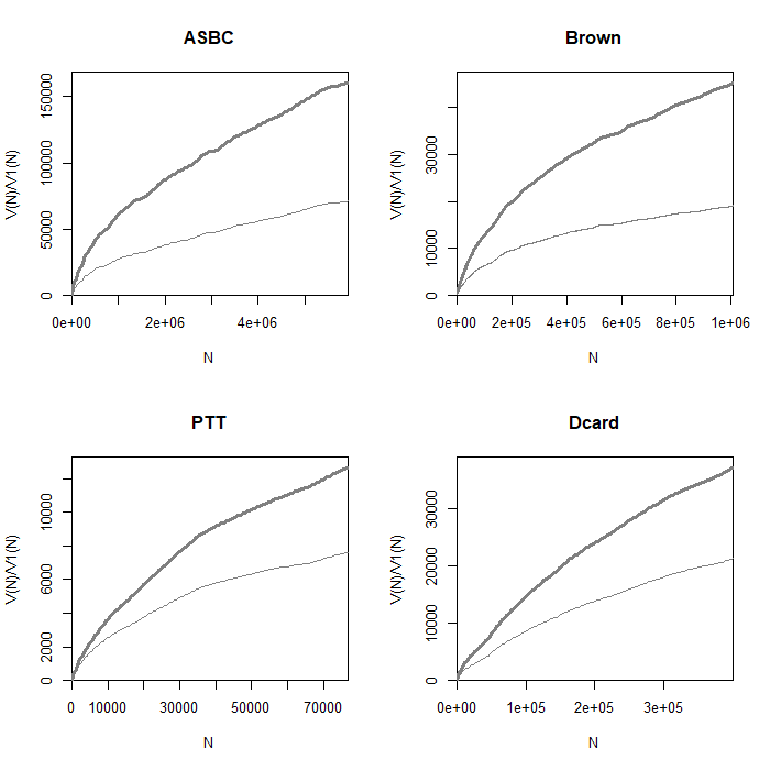
將資料畫成圖表：

1
2
3
4
5
6
7
8
9
par(mfrow=c(2,2))
plot(asbc.vgc, add.m=1, main="ASBC",
        xlab="N", ylab="V(N)/V1(N)")
plot(Brown.emp.vgc, add.m=1, main="Brown",
        xlab="N", ylab="V(N)/V1(N)")
plot(ptt.vgc, add.m=1, main="PTT",
        xlab="N", ylab="V(N)/V1(N)")
plot(dcard.vgc, add.m=1, main="Dcard",
        xlab="N", ylab="V(N)/V1(N)")

上圖中顏色較深的曲線是 V，較淺的曲線是 V1。從圖中可以發現 ASBC 與 Brown corpus 的 V1 曲線上升後逐漸平緩，然而 PTT 與 Dcard 的 V1 曲線呈現持續上升的趨勢，意指隨著 sample size 增加，hapax legomena 也會不斷增加。這可能是中文斷詞錯誤所造成 (Hsieh 2014)。為了推得母體的真實情況，接下來將使用 Large-Number-of-Rare-Events (LNRE) models (Baayen 2002)。

Fitting the LNRE Model

zipfR 套件中提供了三種 LNRE models，分別是 Generalized Inverse Gauss Poisson (lnre.gigp; Baayen, 2001, ch. 4)、Zipf-Mandelbrot (lnre.zm; Evert, 2004)，和 finite Zipf-Mandelbrot (lnre.fzm; Evert, 2004)，我們首先採用 fzm。

 1
 2
 3
 4
 5
 6
 7
 8
 9
10
11
12
13
14
15
16
asbc.fzm <- lnre("fzm", spc=asbc.spc)
Brown.fzm <- lnre("fzm", spc=Brown.spc)
ptt.fzm <- lnre("fzm", spc=ptt.spc)
dcard.fzm <- lnre("fzm", spc=dcard.spc)

# frequency spectrum
asbc.fzm.spc <- lnre.spc(asbc.fzm, N(asbc.spc))
Brown.fzm.spc <- lnre.spc(Brown.fzm, N(Brown.spc))
ptt.fzm.spc <- lnre.spc(ptt.fzm, N(ptt.spc))
dcard.fzm.spc <- lnre.spc(dcard.fzm, N(dcard.spc))

# VGC
asbc.fzm.vgc <- lnre.vgc(asbc.fzm, N(asbc.vgc), m.max=1, variances=TRUE)
Brown.fzm.vgc <- lnre.vgc(Brown.fzm, N(Brown.emp.vgc), m.max=1, variances=TRUE)
ptt.fzm.vgc <- lnre.vgc(ptt.fzm, N(ptt.vgc), m.max=1, variances=TRUE)
dcard.fzm.vgc <- lnre.vgc(dcard.fzm, N(dcard.vgc), m.max=1, variances=TRUE)

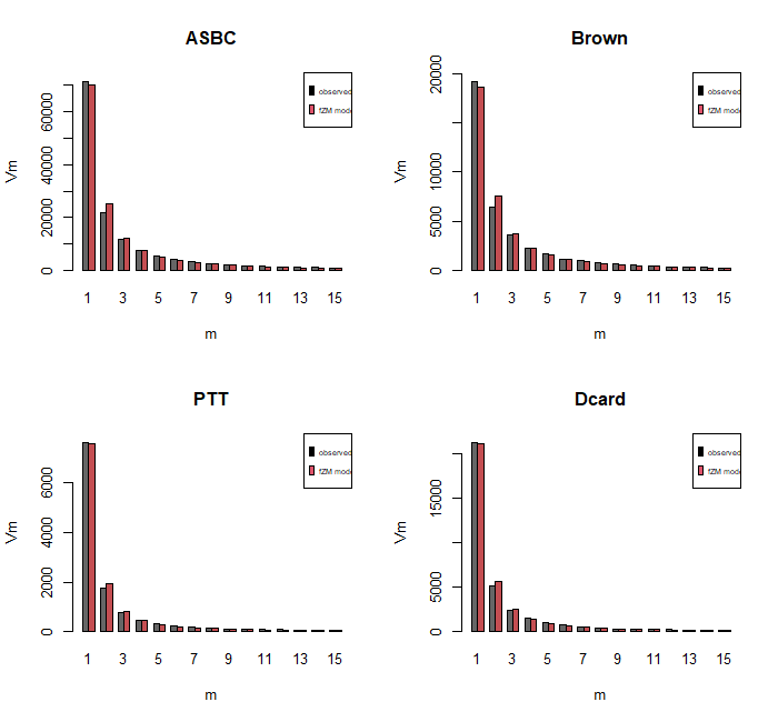
Observed and expected frequency spectra:

 1
 2
 3
 4
 5
 6
 7
 8
 9
10
11
12
13
14
15
16
17
par(mfrow=c(2,2)) 
plot(asbc.spc, asbc.fzm.spc,
        main="ASBC", xlab="m", ylab="Vm")
legend("topright", legend = c("observed", "fZM model"), 
        fill = 1:2, cex = 0.5)
plot(Brown.spc, Brown.fzm.spc,
        main="Brown", xlab="m", ylab="Vm")
legend("topright", legend = c("observed", "fZM model"), 
        fill = 1:2, cex = 0.5)
plot(ptt.spc, ptt.fzm.spc,
        main="PTT", xlab="m", ylab="Vm")
legend("topright", legend = c("observed", "fZM model"), 
        fill = 1:2, cex = 0.5)
plot(dcard.spc, dcard.fzm.spc,
        main="Dcard", xlab="m", ylab="Vm")
legend("topright", legend = c("observed", "fZM model"), 
        fill = 1:2, cex = 0.5)

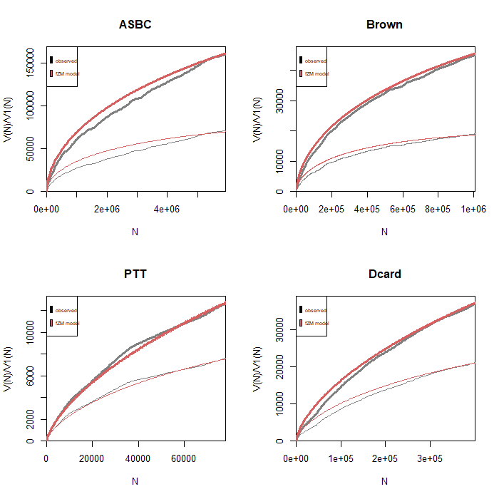
Observed and expected VGC:

 1
 2
 3
 4
 5
 6
 7
 8
 9
10
11
12
13
14
15
16
17
par(mfrow=c(2,2)) 
plot(asbc.vgc, asbc.fzm.vgc, add.m=1,
        main="ASBC", xlab="N", ylab="V(N)/V1(N)")
legend("topleft", legend = c("observed", "fZM model"),
        fill = 1:2, cex = 0.5)
plot(Brown.emp.vgc, Brown.fzm.vgc, add.m=1,
        main="Brown", xlab="N", ylab="V(N)/V1(N)")
legend("topleft", legend = c("observed", "fZM model"),
        fill = 1:2, cex = 0.5)
plot(ptt.vgc, ptt.fzm.vgc, add.m=1,
        main="PTT", xlab="N", ylab="V(N)/V1(N)")
legend("topleft", legend = c("observed", "fZM model"),
        fill = 1:2, cex = 0.5)
plot(dcard.vgc, dcard.fzm.vgc, add.m=1,
        main="Dcard", xlab="N", ylab="V(N)/V1(N)")
legend("topleft", legend = c("observed", "fZM model"),
        fill = 1:2, cex = 0.5)

上方的紅色曲線代表透過 fZM model 所產生的 expected value。

Lexical Coverage Estimation

Out-Of-Vocabulary (OOV) types

我們可以藉由 Out-Of-Vocabulary (OOV) types 的比例來了解兩個 corpus 的 lexical coverage。基本上，一個實用的語言資源中，OOV 所佔的比例應保持在一定標準之下。

我們先採前十萬個 lemma：

1
2
3
4
asbc100k <- head(asbc_corpus, 100000)
data("Brown100k.spc")
ptt100k <- head(ptt_corpus, 100000)
dcard100k <- head(dcard_corpus, 100000)

同樣地，將他們轉成 spc object：

1
2
3
4
5
6
7
asbc100k.tfl <- vec2tfl(asbc100k)
ptt100k.tfl <- vec2tfl(ptt100k)
dcard100k.tfl <- vec2tfl(dcard100k)

asbc100k.spc <- tfl2spc(asbc100k.tfl)
ptt100k.spc <- tfl2spc(ptt100k.tfl)
dcard100k.spc <- tfl2spc(dcard100k.tfl)

首先，我們要計算 lexical of seen types。在這裡，我們將只出現過一次的 type 都算成 OOV。也就是說，我們想要知道語料中至少出現過兩次的 type 總共有幾個：

1
2
3
4
asbc_Vseen <- V(asbc100k.spc) - Vm(asbc100k.spc, 1)
Brown_Vseen <- V(Brown100k.spc) - Vm(Brown100k.spc, 1)
ptt_Vseen <- V(ptt100k.spc) - Vm(ptt100k.spc, 1)
dcard_Vseen <- V(dcard100k.spc) - Vm(dcard100k.spc, 1)

Fitting the LNRE Model

1
2
3
4
asbc100k.fzm <- lnre("fzm", asbc100k.spc)
Brown100k.fzm <- lnre("fzm", Brown100k.spc)
ptt100k.fzm <- lnre("fzm", ptt100k.spc)
dcard100k.fzm <- lnre("fzm", dcard100k.spc)

以 Brown corpus 為例，假設我們用 1, 10, or 100 million tokens 進行計算，expected OOV 分別會是：

 1
 2
 3
 4
 5
 6
 7
 8
 9
10
11
12
13
14
15
16
17
18
19
# ASBC
1 - (asbc_Vseen / EV(asbc100k.fzm, c(1e6, 10e6, 100e6)))

## [1] 0.7751460 0.7844322 0.7844322

# Brown
1 - (Brown_Vseen / EV(Brown100k.fzm, c(1e6, 10e6, 100e6)))

## [1] 0.7299293 0.7347804 0.7347804

# PTT
1 - (ptt_Vseen / EV(ptt100k.fzm, c(1e6, 10e6, 100e6)))

## [1] 0.8847203 0.9098196 0.9098338

# Dcard
1 - (dcard_Vseen / EV(dcard100k.fzm, c(1e6, 10e6, 100e6)))

## [1] 0.8608032 0.8905452 0.8905602

從上方得到的數值可以發現，ASBC 和 Brown corpus 的 OOV ratio 較 PTT 和 Dcard 來得穩定且比例也較低。

結論

利用 zipfR 並採用 LNRE model 對資料進行分析，取得語料的 VGC 和 OOV ratio，就可以分析平衡語料庫、Brown corpus、PTT 和 Dcard 的 lexical richness 和 lexical coverage。目前的發現是：

不同於 ASBC 和 Brown Corpus 最後達成平緩的趨勢，PTT 與 Dcard 的 VGC V1 曲線都隨著 sample size 的增加持續上升。
從 expected OOV ratio 來看，PTT 與 Dcard 語料的 OOV 除比例較高外，也隨著 corpus size 的增加而持續上升，並不如 ASBC 與 Brown corpus 穩定。

可能的原因是，ASBC 是機器斷詞後再進行人工校正而成的語料庫，而 Brown Corpus 是英文語料，字詞與字詞之間已有空白分隔，所以這兩個語料庫較無斷詞錯誤導致新詞不斷增加的問題。然而現今的 Web-as-Corpus，其前處理通常採用機器自動斷詞，龐大的 OOV 可能來自於斷詞錯誤。這說明了在建造中文 Web-as-Corpus 時，斷詞問題是很重要的考量之一。

References

Baayen, R. H. (2002). Word frequency distributions (Vol. 18). Springer Science & Business Media.

Evert S, Baroni M (2007). “zipfR: Word Frequency Distributions in R.” In Proceedings of the 45th Annual Meeting of the Association for Computational Linguistics, Posters and Demonstrations Sessions, 29–32. (R package version 0.6-70 of 2020-10-10).

Kilgarriff, A., & Grefenstette, G. (2003). Introduction to the special issue on the web as corpus. Computational linguistics, 29(3), 333-347.

Hsieh, S.-K. (2014, may). Why Chinese Web-as-Corpus is Wacky? Or: How Big Data is Killing Chinese Corpus Linguistics. Paper presented at the Proceedings of the Ninth International Conference on Language Resources and Evaluation (LREC?14), Reykjavik, Iceland.

Special Thanks

謝謝 Jessy 和 Yongfu 在 HOCOR 2020 提供的 corpus data。

Click here for poster version (made with posterdown)